A SerDes channel typically is a differential signal transmission channel. A hardware SerDes channel is typically characterized by measuring its N-port S-parameters and is typically a 4-port. The 4-port differential input ports are typically port 1 (+) and port 3 (-). The associated differential output ports are typically port 2 (+) and port 4 (-). The differential characteristic ( Port 1 – Port 3 vs. Port 2 – Port 4) is the channel transmission characteristic and is observed versus frequency.
See S-parameter detail in References > S-Parameter Channel Examples.
The eye analysis is performed on the channel that was first analyzed using the Channel Analysis Tool.
The S-parameter file used in the Channel Analysis Tool are automatically adjusted as needed to conform to the physical realizability constraints of passivity, reciprocity, and causality, as well as reduction of noise in the S-parameters. The ports of the S-parameter data are terminated in the characteristic resistance specified in the S-parameter files. Within the Channel Analysis Tool an optimal FFE is applied to open the channel eye performance.
Once the channel with optimal FFE equalization is analyzed, the Eye Analysis Tool provides detail channel eye analysis, including jitter and BER analysis, The Eye Analysis Tool uses the channel characteristics obtained using the Channel Analysis Tool.
See About the Eye Analysis Tool for setup and use of this tool.
For the example channel with optimal FFE equalization applied, several graphical displays available are shown here for BitRate = 25Gbps, SamplesPerBit = 32, Tx_Dj = Tx_Rj = Rx_Dj = Rx_Rj = 0.25 psec and time display (x-axis) in time sec units.
Figure 1. Impulse response for channel with optimal FFE equalization (3 pre-cursors, 5 post-cursors).
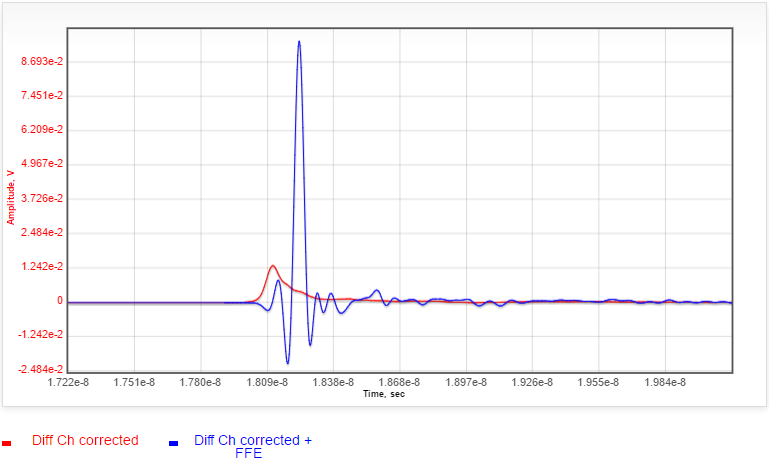
These impulse responses were obtained using the Channel Analysis Tool. The red curve is for the channel without equalization. The channel inherently has a delay of about 18 nsec. The blue curve is for the channel equalized using an optimal FFE.
Figure 2. Eye worst/best case contours without jitter.
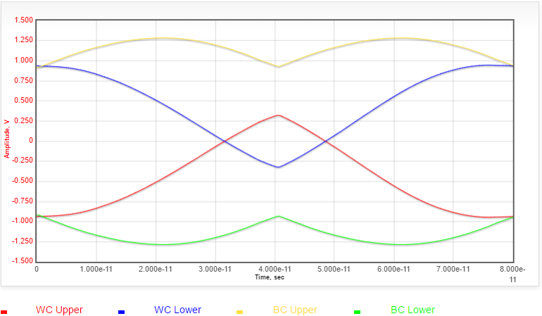
These best/worst case eye contours are based on a statistical analysis of the impulse response and effectively is for a bit stream as long as the impulse response and inclusive of all possible pit patterns for that bit stream. The x-axis spans a two bit timing interval (80 psec).
Figure 3. Eye density plot
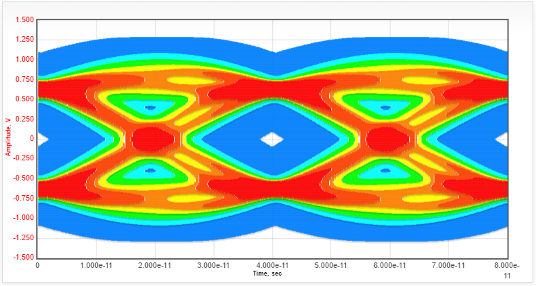
This eye density plot is inclusive of all the jitter. Each color represents a different eye density. Blue represents the least dense eye. Red represents the most dense eye. Observe that the eye is much closed due to the jitter compared to the previous plot for the best/worst case eye contours with no jitter. The x-axis spans a two bit timing interval (80 psec).
Figure 4. Jitter PDF
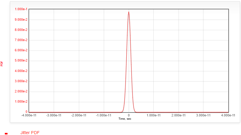
This jitter shown in this plot is what causes the eye closure in the previous plot for the eye density with jitter.
Figure 5. Eye amplitude bathtub BER
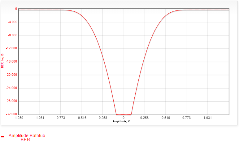
This BER plot versus amplitude is at the timing instant specified which was at the eye timing center. The amplitude spans the range from the lowest eye amplitude value to the largest amplitude value as seen in the prior eye density plot.
Figure 6. Eye timing bathtub BER
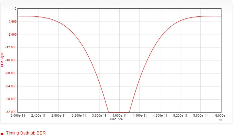
This BER plot versus time is at the amplitude level specified which was at 0 V. The time spans the range about the center of the eye density plot by -/+ 0.5 bit time.
Figure 7. BER vs eye height
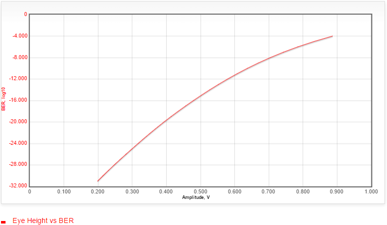
This plot shows the open eye amplitude height at various BER levels measured at the timing instant specified which was at the eye timing center. The eye width was based on the measurement option selected which was Right + Left amplitude bathtub BER curve value distance at SamplingTOffset.
Figure 8. BER vs eye width
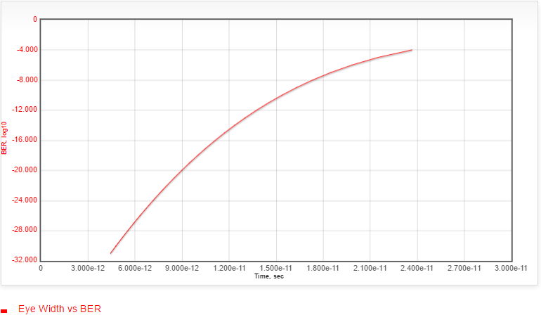
This plot shows the open eye time width at various BER levels measured at the voltage instant specified which was 0 V. The eye width was based on the measurement option selected which was Right + Left timing bathtub BER curve value distance at SamplingVOffset.